Social media analysis (using APIs Meta & X)

Important

En esta oportunidad se trabajan con datos extraídos a través de la API de Meta y X. Lo único que se necesita son las credenciales y claves Key que genera y proporciona cada plataforma. Antes de poder acceder a cualquiera de las claves y servicios, es necesario solicitar una autorización en el sitio web de desarrolladores de Meta y X.

La extracción de datos por estas vías están sujetas a las regulaciones de cada plataforma (se obtienen métricas en tiempo real, comentarios, urls y datos en tiempos especificos). Esta vez el compendio está desarrollado con Python (extracción) y R (manipulación de datos y gráficos) Este panel de control se ha creado en quarto. Se extrae la data y se actualiza el gráfico dinámicamente. Las APIs se ejecutan automáticamente tres veces por mes, puede configurarse al momento de crear las claves API y las peticiones de consulta, hay diferentes límites de tiempo disponibles.

Ejemplo: API; https://github.com/freddyvillabona/extraer-tuits-tweepy/tree/master

Important

In this instance, we are working with data extracted via the Meta and X APIs. All you need are the credentials and K keys generated by each platform. Before you can access any of the keys, you must request authorisation from the Meta and X developer websites.

Built with Python and R. This dashboard is created in Quart. The API runs the queries three times a month.

APIs: https://github.com/freddyvillabona/extraer-tuits-tweepy/tree/master

# LIBRARIES
library(tidyverse)
library(ggpubr)
library(reshape2)
library(ggcorrplot)
library(ggcharts)
library(tmaptools)
library(prismatic)
library(patchwork)
library(gridExtra)
library(ggflags)
library(showtext)
library(camcorder)
library(ggtext)


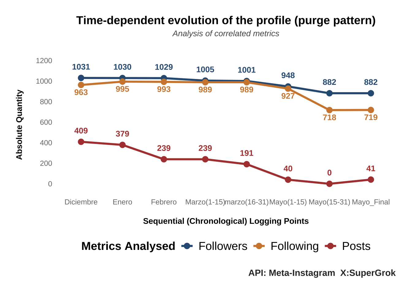
datos <- data.frame(
  Mes = factor(rep(c("Diciembre", "Enero", "Febrero", "Marzo(1-15)", "marzo(16-31)", "Mayo(1-15)", "Mayo(15-31)", "Mayo_Final"), 3),
               levels = c("Diciembre", "Enero", "Febrero", "Marzo(1-15)", "marzo(16-31)", "Mayo(1-15)", "Mayo(15-31)", "Mayo_Final")),
  Metrica = rep(c("Followers", "Following", "Posts"), each = 8),
  Cantidad = c(
    # Seguidores (8 elementos)
    1031, 1030, 1029, 1005, 1001, 948, 882, 882,
    # Seguidos (8 elementos)
    963, 995, 993, 989, 989, 927, 718, 719,
    # Publicaciones (8 elementos)
    409, 379, 239, 239, 191, 40, 0, 41
  ),
  # Ajuste vertical adaptado para las 3 métricas (8 elementos por bloque, total 24)
  vjust_personalizado = rep(c(-1.5, 1.8, -1.5), each = 8)
)

# 2. Definición de la paleta de colores
colores_personalizados <- c(
  "Followers" = "#2E5B82",    # Azul sutil
  "Following" = "#D0873D",    # Naranja/Dorado
  "Posts" = "#B0413E"         # Rojo/Marrón opaco
)


# FONTS
font_add_google("Luckiest Guy","ramp")
font_add_google("Bebas Neue","beb")
font_add_google("Fira Sans","fira")
font_add_google("Raleway","ral")
font_add_google("Bitter","bit")
showtext_auto()

# 2. Definición de la paleta de colores
colores_personalizados <- c(
  "Followers" = "#2E5B82",    # Azul sutil
  "Following" = "#D0873D",    # Naranja/Dorado
  "Posts" = "#B0413E"         # Rojo/Marrón opaco
)

# 3. Construcción del gráfico con ggplot2
ggplot(datos, aes(x = Mes, y = Cantidad, group = Metrica, color = Metrica)) +
  
  # Líneas y puntos con los grosores correspondientes
  geom_line(linewidth = 1.2) +
  geom_point(size = 3) +
  
  # Etiquetas de texto con posición dinámica y tipografía en negrita
  geom_text(aes(label = Cantidad, vjust = vjust_personalizado),
            fontface = "bold",
            size = 3.5,
            show.legend = FALSE) +
  
  # Escala de colores manual
  scale_color_manual(values = colores_personalizados, name = "Metrics Analysed") +
  
  # Ajuste de los límites y cortes del eje Y
  scale_y_continuous(limits = c(-50, 1200), breaks = seq(0, 1200, by = 200)) +
  
  # Títulos y etiquetas de los ejes
  labs(
    title = "Time-dependent evolution of the profile (purge pattern)",
    subtitle = "Analysis of correlated metrics",
    caption = "API: Meta-Instagram  X:SuperGrok",
    x = "Sequential (Chronological) Logging Points",
    y = "Absolute Quantity"
  ) +
  

  theme_minimal() +
  theme(
    plot.caption = element_text(face = "bold", size = 11, color = "#333333", margin = margin(t = 15)),
    plot.title = element_text(face = "bold", size = 14, hjust = 0.5, margin = margin(b = 5)),
    plot.subtitle = element_text(face = "italic", size = 10, hjust = 0.5, color = "#555555", margin = margin(b = 20)),
    axis.title.x = element_text(face = "bold", size = 10, margin = margin(t = 15)),
    axis.title.y = element_text(face = "bold", size = 10, margin = margin(r = 15)),
    axis.text = element_text(color = "#777777", size = 9),
    
    panel.grid.major = element_line(color = "#FFFFFF", linetype = "dashed"),
    panel.grid.minor = element_blank(),
    

    legend.position = "bottom",
    legend.direction = "horizontal",
    legend.title = element_text(size = 14, face = "bold"), 
    legend.text = element_text(size = 14),                
    legend.spacing.x = unit(0.3, "cm"),                  
    plot.margin = margin(20, 20, 20, 20)
  )

La Psicología y la Ciencia de Datos tienen lazos muy importantes en la búsqueda de patrones. Este gráfico estadístico trabajado con regresión lineal múltiple y datos reales, representa un evento denominado —Tierrra Quemada—: ocurrido con un paciente después de un colapso emocional por carga de culpa,miedo a la soledad, presión, evasión, conflictos internos no resueltos y huida hacia adelante en complicidad.

Un análisis psicológico de María José Valiente por este caso con una metáfora. «Es algo como ejecutar un disparo y después ocultar el arma debajo de la alfombra, lavarse las manos y huir en cómplicidad. Hay que desaparecer cualquier rastro digital, especialmente en redes sociales para no sentir. Solapar nexos y suprimir el pasado para poder vivir y no herir al entorno, tácticamente fingir ante los demás: aquí no ha pasando nada es solo un movimiento pequeño». —María José Valiente

Investigación realizada con Python, R APIs Meta & X.