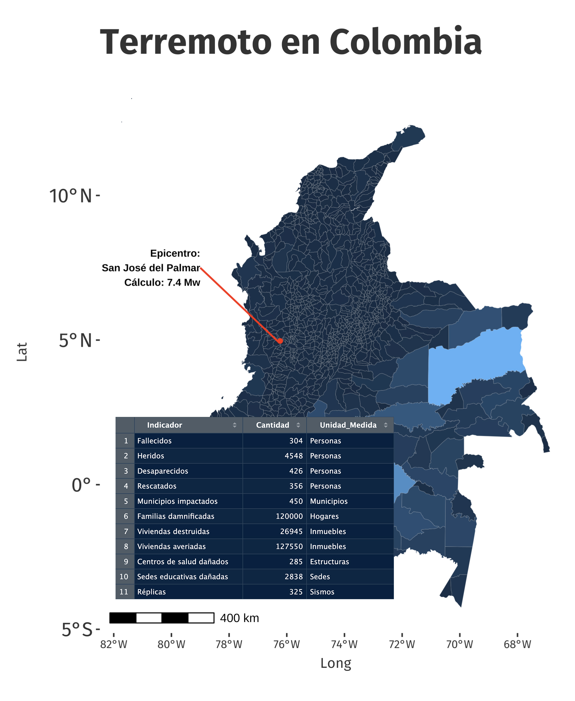
Haz clic aquí para ver las 200 líneas de código
{
library("rvest")
library('sf')
library("ggplot2")
library("tmap")
library("unikn")
library("dplyr")
library("showtext")
library("unikn")
library("tidyverse")
library("mapchina")
library("ggspatial")
}

font_add_google("Fira Sans","fira")
showtext_auto()
map <- read_sf('shapes.shp')

g <- filter(map, nombre_mpi %in% c("CUMARIBO",
                                   "SOLANO",
                                   "SAN JOSE DEL GUAVIARE",
                                   "LA PRIMAVERA",
                                   "PUERTO SANTANDER"))
g <- g[-4,]


paleta <- c("red","blue")
paleta <- unikn::usecol(paleta, n=5)


paleta <- RColorBrewer::brewer.pal(9, "Blues")
paleta
paleta <- paleta[4:9]

paleta2 <- head(rev(RColorBrewer::brewer.pal(9, "Blues")),5)


bubble_sizes <- c(1,1,1,1,1)
punto <- "Municipios más extensos"


mapa <- tm_shape(map)+
  tm_fill(col = "area", palette = paleta, style = "kmeans",
          colorNA = "snow3", title = "Área (km²)"
          ) +
  tm_borders("grey90", lwd = 0.002)+
  #tm_graticules(col = "grey90")+
  tm_scalebar(position = c("left", "bottom"))+
  tm_layout(title = "Municipios de Colombia (área en km²)",
            title.size=2,
            bg.color ="#f8f8f8",
            title.bg.color = "#f0f0f0",
            #title.position = "TOP"
            title.position = c("left", 'top')

            ) +

  tm_shape(g)+
  #tm_style_white("A map with bold title", frame = F, fontface=2) +
  tm_text(text="nombre_mpi",
          size = .7,
          col = "#f8f8f8") +

  #tm_shape(geocode2) +      # dots shape
  #tm_dots(col = "red", size = .1) +

  tm_add_legend('symbol',
                col="#08306B",
                border.col = "white",
                lwd = 0.001,
                labels = c(" Total de municipios: 1103")
  ) +

  tm_add_legend('symbol',
                #col = head(rev(RColorBrewer::brewer.pal(9, "YlGnBu") ),5 ),
                col = paleta2,
                border.col = "grey40",
                size = bubble_sizes,
                labels = c('1: Cumaribo, Vichada',
                           '2: Solano, Caqueta',
                           "3: San José, Guaviare",
                           '4: La Primavera, Vichada',
                           "5: Pto. Santander, Amazonas"),
                title=punto
                ) +


  tm_credits("Datos: opendatasoft",
             position=c("left", "bottom"))


mapa


a <- tmap::tmap_leaflet(mapa)

a
 #GGPLOT2

ru <- map %>%
  st_as_sf()

ru$area

A <- ggplot(data = ru) +
  ggtitle("Terremoto en Colombia") +
  xlab("Lat") +
  ylab("Long") +
  geom_sf(aes(fill=area), show.legend = T, size = 0.05) +
  theme(plot.title = element_text(size = 16),
        plot.subtitle = element_text(size = 20)) +
  annotation_scale() +
  theme(text = element_text(family = "fira"),
        panel.grid = element_blank(),
        plot.title = element_text(size = 25, colour = "gray20", face="bold"),
        axis.text.y = element_text(size = 8, colour = "gray20"),
        axis.title.x = element_text(size = 18, colour = "gray20"),
        axis.title.y = element_text(size = 8, colour = "gray20"),
        axis.text.x = element_text(size = 8, colour = "gray20"),
        panel.background = element_rect(fill = 'white', color = 'white'),
        legend.position = "none")

A

A <- ggplot(data = ru) +
  ggtitle("Terremoto en Colombia") +
  xlab("") + ylab("") +
  # SOLUCIÓN: fill y color configurados por fuera de aes()
  geom_sf(fill = "red", color = "gray40", size = 0.05) +
  theme(plot.title = element_text(size = 16), plot.subtitle = element_text(size = 20)) +
  annotation_scale() +
  theme(text = element_text(family = "fira"),
        panel.grid = element_blank(),
        plot.title = element_text(size = 25, colour = "gray20", face = "bold"),
        axis.text.y = element_text(size = 8, colour = "gray20"),
        axis.title.x = element_text(size = 18, colour = "gray20"),
        axis.title.y = element_text(size = 8, colour = "gray20"),
        axis.text.x = element_text(size = 8, colour = "gray20"),
        panel.background = element_rect(fill = 'white', color = 'white'),
        legend.position = "none")

A


A <- ggplot(data = ru) +
  ggtitle("Terremoto en Colombia") +
  xlab("") + ylab("") +
  # SOLUCIÓN: fill = NA (transparente) y color = "red" (borde)
  geom_sf(fill = NA, color = "red", size = 0.2) +
  theme(plot.title = element_text(size = 16), plot.subtitle = element_text(size = 20)) +
  annotation_scale() +
  theme(text = element_text(family = "fira"),
        panel.grid = element_blank(),
        plot.title = element_text(size = 25, colour = "gray20", face = "bold"),
        axis.text.y = element_text(size = 8, colour = "gray20"),
        axis.title.x = element_text(size = 18, colour = "gray20"),
        axis.title.y = element_text(size = 8, colour = "gray20"),
        axis.text.x = element_text(size = 8, colour = "gray20"),
        panel.background = element_rect(fill = 'white', color = 'white'),
        legend.position = "none")

A


pb <- data.frame(long = -76.23, lat = 4.97)


A <- ggplot(data = ru) +
  ggtitle("Terremoto en Colombia") +
  xlab("Long") + ylab("Lat") +
  # SOLUCIÓN: aes(fill=area) mantiene tus colores internos, color="red" cambia los bordes
  geom_sf(aes(fill = area), color = "white", size = 0.02, show.legend = TRUE) +
  theme(plot.title = element_text(size = 16), plot.subtitle = element_text(size = 20)) +
  annotation_scale() +
  annotate("segment",
           x = -80.0, y = 6.5,         # Coordenadas de inicio (donde estará el texto)
           xend = -76.25, yend = 4.9,   # Coordenadas del epicentro (punto rojo)
           color = "red",
           linewidth = 0.6,
           arrow = arrow(length = unit(0.2, "cm"))) + # Agrega una flecha en la punta

  # 2. Agregar la etiqueta de texto
  annotate("text",
           x = -80.2, y = 6.5,         # Ubicación del texto (alineado con la línea)
           label = "Epicentro:\nSan José del Palmar",
           color = "black",
           fontface = "bold",
           size = 1,
           hjust = 1) +
  geom_point(data = pb, aes(x = long, y = lat),
             color = "red", size = 0.9, shape = 19) +
  theme(text = element_text(family = "fira"),
        panel.grid = element_blank(),
        plot.title = element_text(size = 25, colour = "gray20", face = "bold"),
        axis.text.y = element_text(size = 14, colour = "gray20"),
        axis.title.x = element_text(size = 10, colour = "gray20"),
        axis.title.y = element_text(size = 10, colour = "gray20"),
        axis.text.x = element_text(size = 8, colour = "gray20"),
        panel.background = element_rect(fill = 'white', color = 'white'),
        legend.position = "none")

A