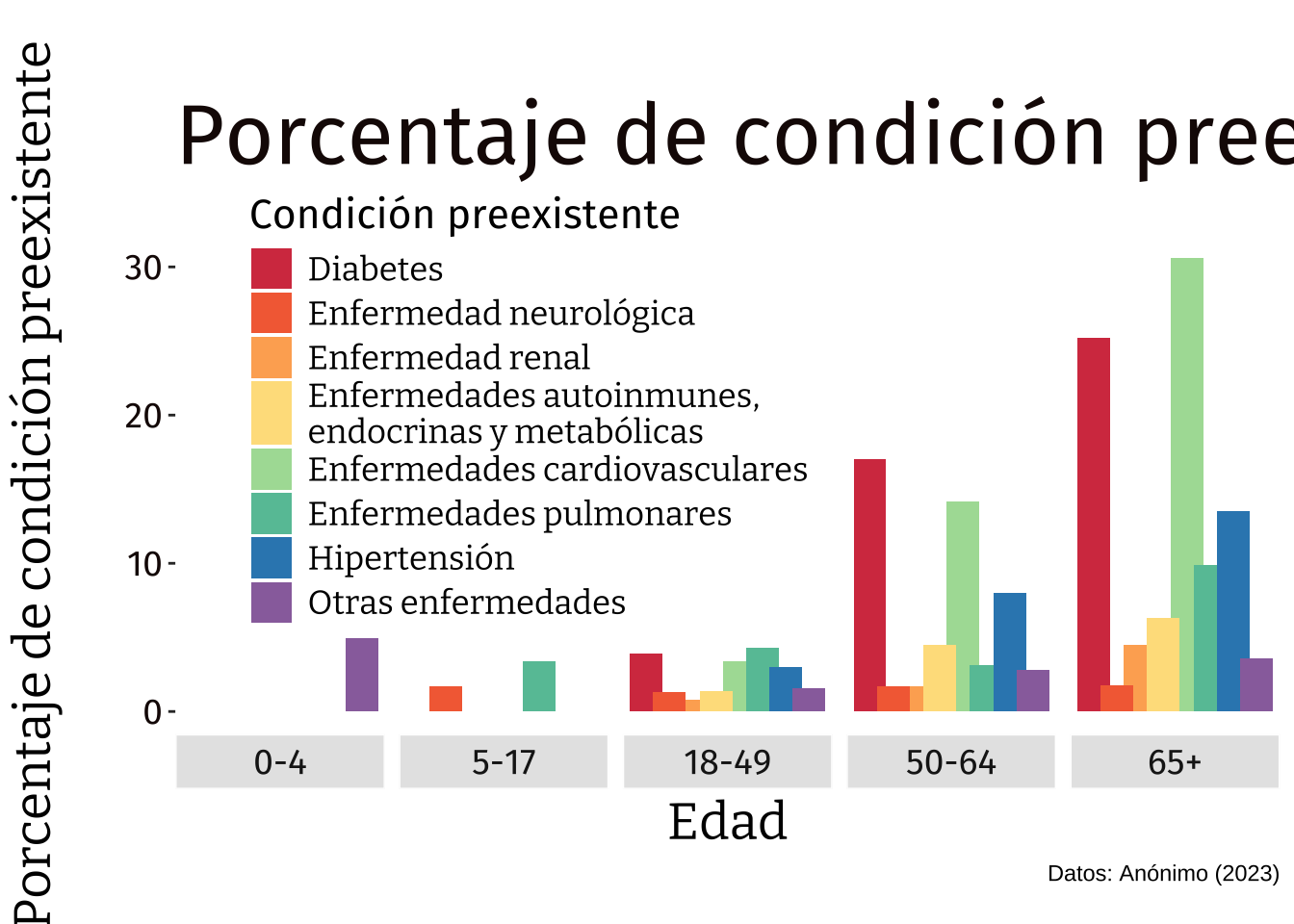
Esta vez se tiene un gráfico de barras “ggplot2” con paleta de colores manual.
Se muestran las categorías por edad de un grupo de enfermedades preexistentes. Además se posiciona la leyenda en la parte superior izquierda. Se usa una paleta de colores personalizada
Code
library("showtext")library("dplyr")library("ggplot2")# FONTSfont_add_google("Luckiest Guy","ramp")font_add_google("Bebas Neue","beb")font_add_google("Fira Sans","fira")font_add_google("Raleway","ral")font_add_google("Bitter","bit")showtext_auto()data <-read.csv("data.csv")ggplot(data,aes(x = Cond_pre, y = Freq, fill = Cond_pre)) +geom_col(width =1.4, just =0.5) +facet_grid(~factor(Age, levels=c("0-4", "5-17", "18-49", "50-64", "65+")),space ="free_x", scales ="free_x", switch ="x")+scale_x_discrete(name ="Edad", expand =c(0, 1)) +ylab("Porcentaje de condición preexistente\n") +scale_fill_manual(values =c("#d53e4f", "#f46d43", "#fdae61", "#fee08b","#abdda4", "#66c2a5", "#3288bd", "#9970ab")) +labs(title="\nPorcentaje de condición preexistente", subtitle ="",caption ="Datos: Anónimo (2023)\n",fill="Condición preexistente") +theme(strip.background =element_rect(color="white", fill="gray90", linetype="solid"), strip.text.x =element_text(size=14, family ="fira"), axis.text.x =element_blank(), axis.ticks.x =element_blank(),panel.grid.major.x =element_blank(),panel.background =element_rect(fill ="white", colour ="white"),legend.position =c(.32, .65),panel.grid.major =element_line(linewidth =0.1, linetype ='solid',colour ="white"), panel.grid.minor =element_line(linewidth =0.1, linetype ='solid',colour ="white"),legend.text =element_text(size=13, family ="bit"), legend.title =element_text(size=16, family ="fira"),axis.title.x=element_text(size=20, family ="bit"),axis.title.y=element_text(size=20, family ="bit"),plot.title=element_text(size=33, family ="fira", color ="#190706"),axis.text.y =element_text(color ="#190706", size=14, family ="fira"),)