Map of the United Kingdom drawn from a shapefile layer. This is a post with executable code.
Code
# LIB
library("dplyr")
library("ggplot2")
library("sf")
library("ggtext")
# UK SHAPEFILE
uk <- read_sf('uk/uk_shapefile.shp')
uk <- uk %>%
st_as_sf()
# DATA (CSV)
data <- read.csv2("data.csv")
# (SHAPEFILE AND DATOS)
map_uk <- merge(uk, data, by = "Region")
map_uk <- map_uk %>%
st_as_sf()
# COLORS
pal <- colorRampPalette(c("#ffffcc", "#c7e9b4", "#7fcdbb",
"#41b6c4", "#2c7fb8"))(12)
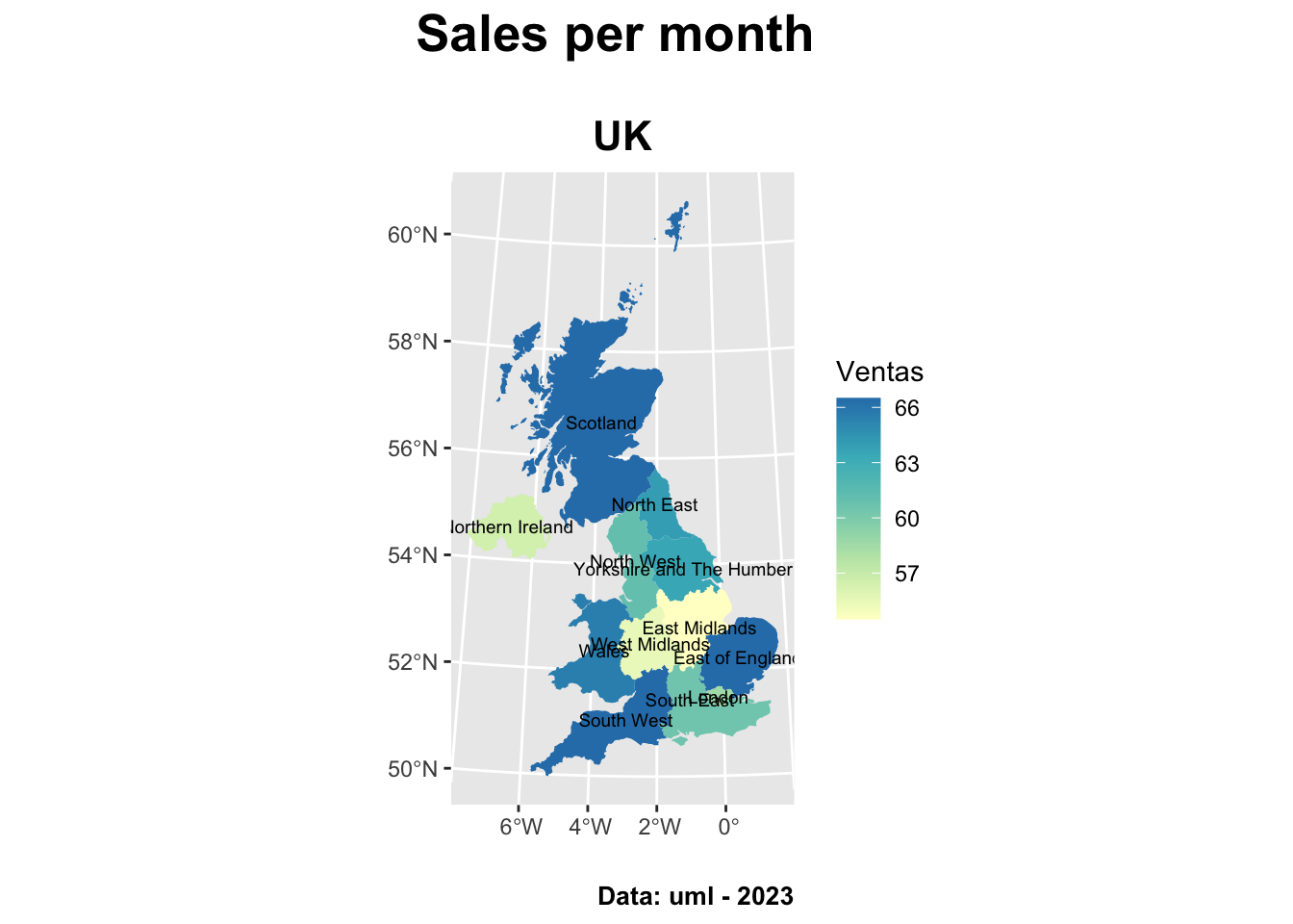
# MAP1
ggplot(data = map_uk) +
xlab("") +
ylab("") +
geom_sf(aes(fill=Mean), show.legend = T, size = 0.05, lwd = 0) +
scale_fill_gradientn(colours = pal) +
geom_sf_text(aes(label =Region),size=2.5, colour="black")+
theme(plot.title = element_text(size = 20, face="bold", hjust = 0.5),
plot.subtitle = element_text(size = 16, face="bold", hjust = 0.5),
plot.caption = element_text(size = 10, face="bold", hjust = 1)) +
labs(title="Sales per month ",
subtitle = "\nUK",
caption = "Data: uml - 2023",
fill= "Ventas")
Code
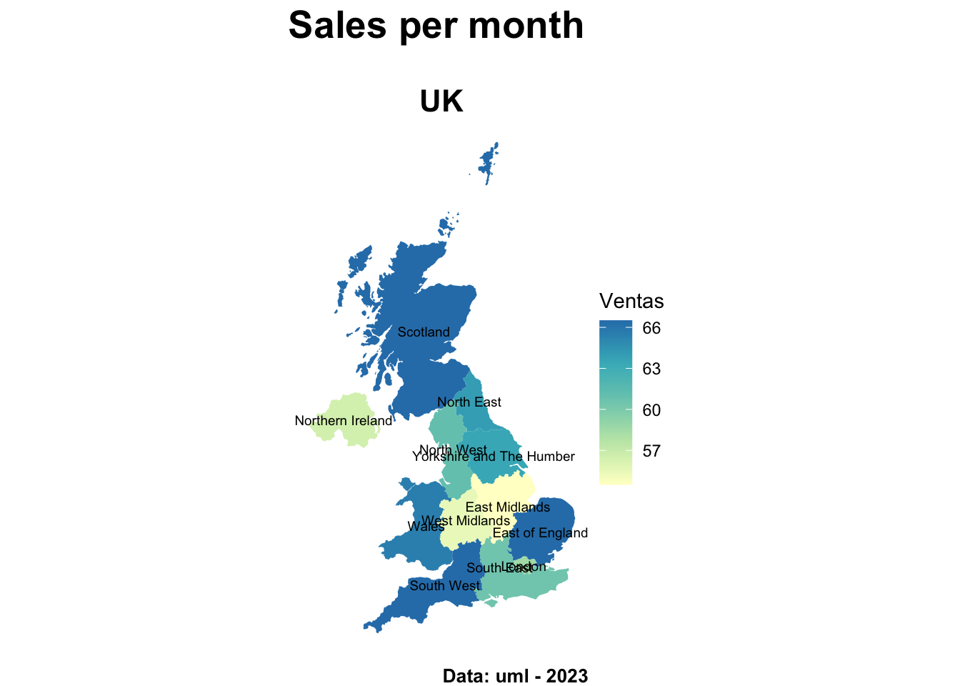
# MAP2

 ggplot(data = map_uk) +
  xlab("") +
  ylab("") +
  geom_sf(aes(fill=Mean), show.legend = T, size = 0.05, lwd = 0) +
  scale_fill_gradientn(colours = pal) +
  geom_sf_text(aes(label =Region),size=2.5, colour="black")+
  theme_void() +
   theme(plot.title = element_text(size = 20, face="bold", hjust = 0.5),
         plot.subtitle = element_text(size = 16, face="bold", hjust = 0.5),
         plot.caption = element_text(size = 10, face="bold", hjust = 1)) +
   labs(title="Sales per month ",
        subtitle = "\nUK",
        caption = "Data: uml - 2023",
        fill= "Ventas")