Población de China

En este caso trabajando con la librería “mapchina”. Esta librería contiene capas shapefile y datos poblacionales. Trabajando con la función gradiente de colores.

Este mapa intenta mostrar algunos detalles significativos al momento de trazar mapas con ggplot2:

• Gradiente de colores (mayor o menor densidad poblacional)
• Trazo de segmentos, puntos y textos en ubicaciones específicas
• Tema personalizado (fondos, fuentes, márgenes, leyendas)

{
library(showtext)
library(unikn)
library(tidyverse)
library(mapchina)
library(sf)
library(ggspatial)
}

font_add_google("Fira Sans","fira")
showtext_auto()

s <- data.frame(x1 = 99, x2 = 127.5, y1 = 26, y2 = 50)

china <- china
df <- china 


plot <- ggplot(data = df) +
  ggtitle("   Población de China") +
  xlab("")+
  ylab("") +
  
  geom_sf(aes(fill = rank(Density)), linewidth = .1) +
  
  scale_fill_gradient2(
    name = waiver(),
    low = "red",
    mid = "#f9f8f9",
    high = "blue",
    midpoint = 0,
    space = "Lab",
    na.value = "grey50",
    transform = "identity",
    guide = "colourbar",
    aesthetics = "fill"
  ) +
  
  geom_text(
            label="94%",
            x = 115, y = 30,
            size = 12,
            family="fira",
            fontface="bold",
            colour = "gray20") +
  
  geom_text(
    label="vive aquí",
    x = 115, y = 28,
    size = 6,
    family="fira",
    colour = "gray20") +
  
  geom_text(
    label="4%",
    x = 90, y = 40,
    size=12,
    family="fira",
    fontface="bold",
    colour = "gray20") +
  
  geom_text(
    label="vive aquí",
    x = 90, y = 38,
    size=6,
    family="fira",
    colour = "gray20") +
  
  
  geom_text(
    label="Población: 1.411.750.000 habs.",
    x = 90, y = 52,
    size=4,
    family="fira",
    colour = "gray20") +
 
  geom_segment(data = s,
               aes(x = x1, y = y1, xend = x2, yend = y2),
               linewidth=1.5, colour = "#fa4c35") +
  
  geom_point(data = s,
               aes(x = x1, y = y1,
                   size=1.8), colour = "#fa4c35") +
  
  geom_text(
    label="Tengchong",
    x = 95, y = 26,
    size = 4,
    family="fira",
    colour = "gray20") +
  
  
  geom_point(data = s,
             aes(x = x2, y = y2,
                 size=1.8), colour = "#fa4c35") +
  
  
  geom_text(
    label="Heihe",
    x = 130, y = 50,
    size = 4,
    family="fira",
    colour = "gray20") +
  
  
  
  theme(plot.title = element_text(size = 30, face = "bold"),
        plot.subtitle = element_text(size = 20),
        legend.position="bottom") +
  labs(fill= "%") +

  annotation_scale() +
  
  theme(text = element_text(family = "fira"),
        panel.grid = element_blank(),
        plot.title = element_text(size = 25, colour = "gray20", face="bold"),
        axis.text.y = element_text(size = 8, colour = "gray20"),
        axis.title.x = element_text(size = 18, colour = "gray20"),
        axis.title.y = element_text(size = 8, colour = "gray20"),
        axis.text.x = element_text(size = 8, colour = "gray20"),
        panel.background = element_rect(fill = 'white', color = 'white'),
        legend.position = "none") 

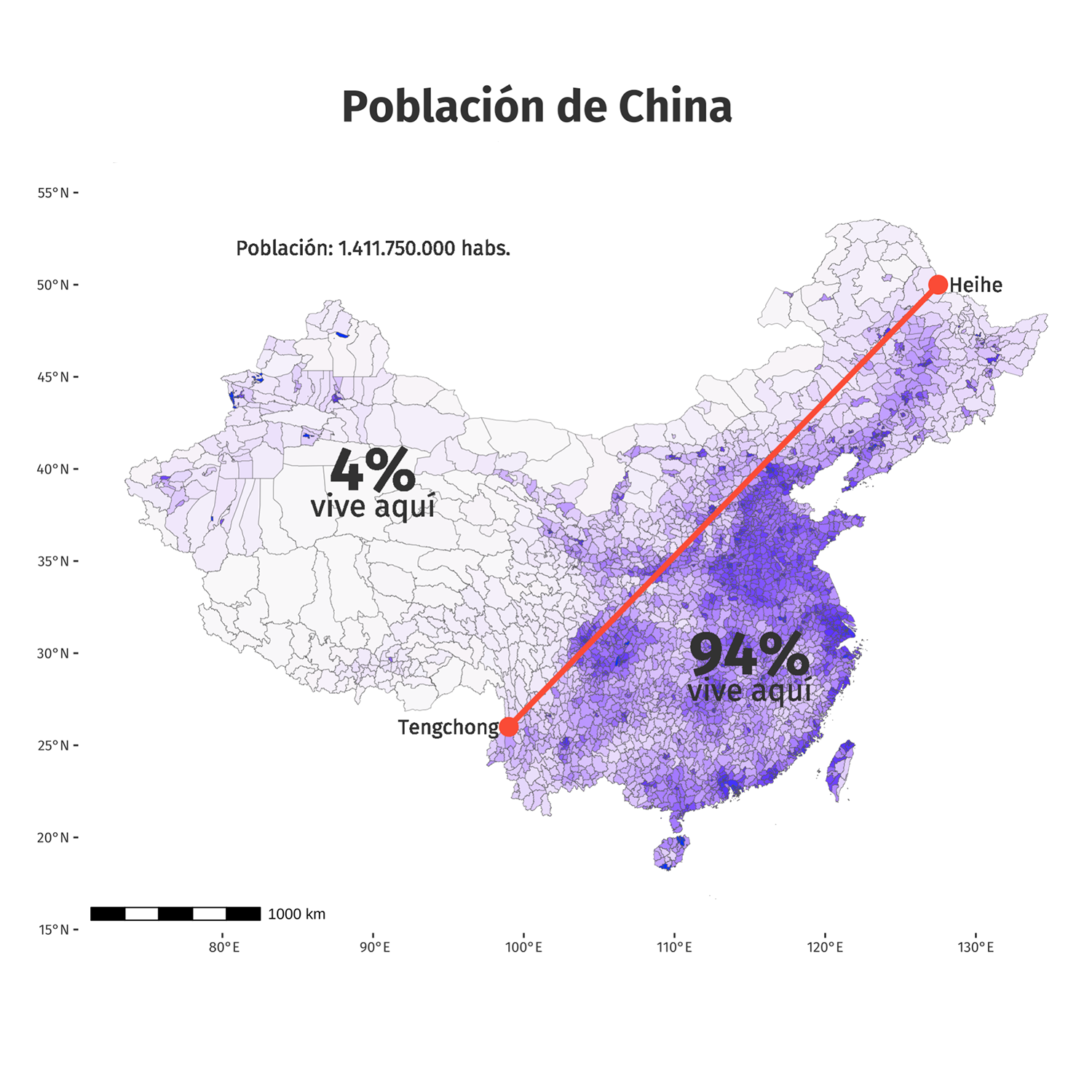
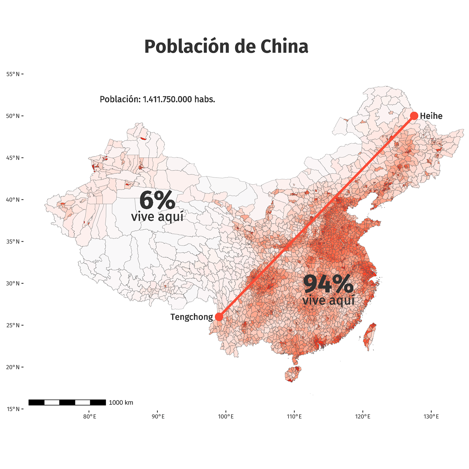
Datos y capa shapefile: library(“mapchina”)