library(tidyverse)
library(showtext)
library(camcorder)
library(ggtext)
#library(nrBrand)
library(glue)
library(ggHoriPlot)
library(PrettyCols)
# Load data ---------------------------------------------------------------
tuesdata <- tidytuesdayR::tt_load("2025-07-01")
weekly_gas_prices <- tuesdata$weekly_gas_prices
# Load fonts --------------------------------------------------------------
font_add_google("Space Grotesk", "space")
showtext_auto()
showtext_opts(dpi = 300)
# Define colours and fonts-------------------------------------------------
bg_col <- "transparent"
text_col <- prettycols("RedBlues")[9]
highlight_col <- prettycols("RedBlues")[1]
body_font <- "space"
title_font <- "space"
# Data wrangling ----------------------------------------------------------
# price data
price_data <- weekly_gas_prices |>
mutate(
year = year(date),
week = week(date)
) |>
filter(fuel == "gasoline", grade == "regular", formulation == "all") |>
select(year, week, price) |>
complete(year, week)
# horizon plot data
cutpoints <- price_data |>
mutate(
outlier = between(
price,
quantile(price, 0.25, na.rm = TRUE) -
1.5 * IQR(price, na.rm = TRUE),
quantile(price, 0.75, na.rm = TRUE) +
1.5 * IQR(price, na.rm = TRUE)
)
) |>
filter(outlier)
ori <- sum(range(cutpoints$price)) / 2
sca <- seq(range(cutpoints$price)[1],
range(cutpoints$price)[2],
length.out = 7
)[-4]
# Start recording ---------------------------------------------------------
gg_record(
dir = file.path("2025", "2025-07-01", "recording"),
device = "png",
width = 5,
height = 14,
units = "in",
dpi = 300
)
# Define text -------------------------------------------------------------
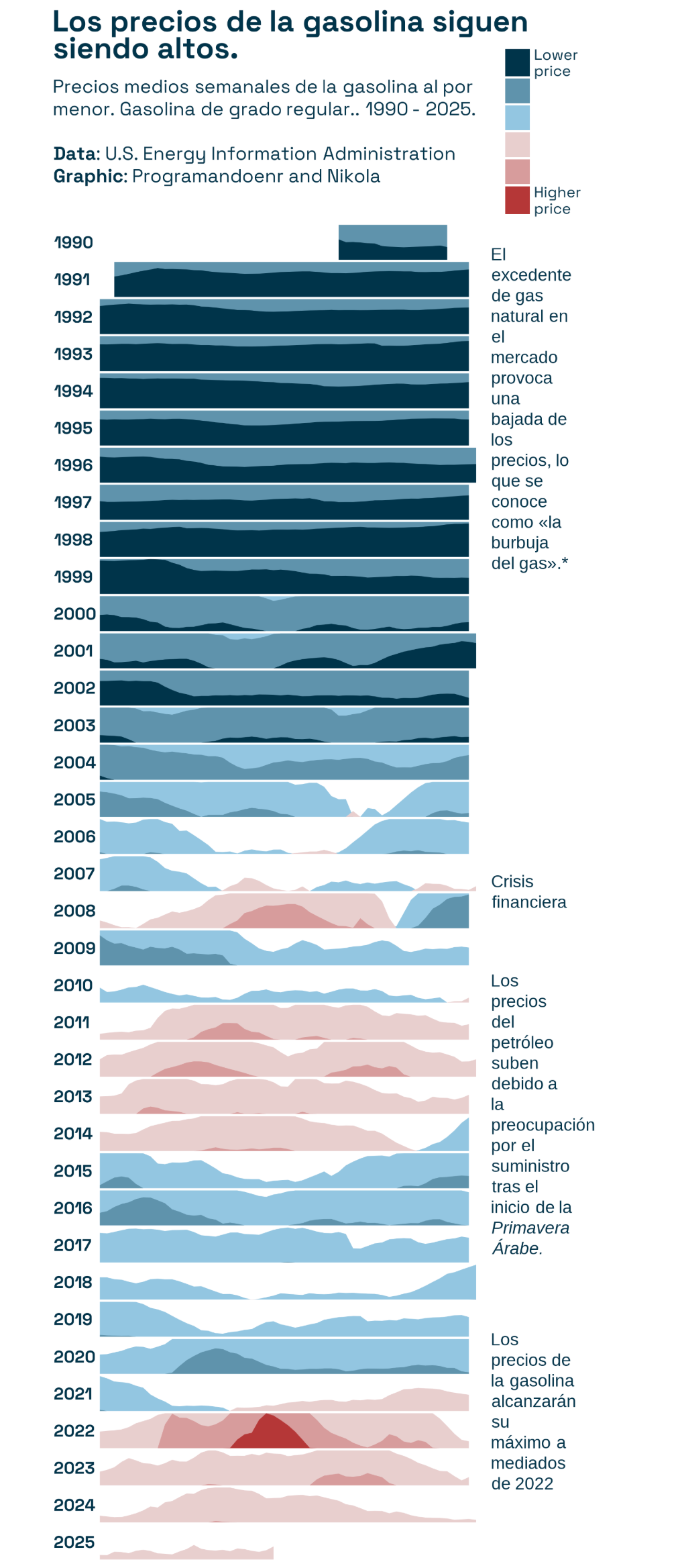
title <- "Los precios de la gasolina siguen siendo altos."
st <- "Precios medios semanales de la gasolina al por menor. Gasolina de grado regular.. 1990 - 2025."
cap <- paste0(
st, "<br><br>**Data**: U.S. Energy Information Administration<br>**Graphic**: ", "Programandoenr and Nikola"
)
# Plot --------------------------------------------------------------------
ggplot(data = price_data) +
geom_horizon(
mapping = aes(
x = week,
y = price,
fill = after_stat(Cutpoints)
),
origin = ori, horizonscale = sca
) +
# annotations
geom_textbox(
data = data.frame(
x = 54, y = 1,
label = "El excedente de gas natural en el mercado provoca una bajada de los precios, lo que se conoce como «la burbuja del gas».*",
year = 1995
),
mapping = aes(x = x, y = y, label = label),
fill = bg_col,
box.color = "transparent",
color = text_col,
halign = 0,
hjust = 0,
maxwidth = 0.2
) +
geom_textbox(
data = data.frame(
x = 54, y = 1, label = "Crisis financiera", year = 2008
),
mapping = aes(x = x, y = y, label = label),
fill = "transparent",
box.color = "transparent",
color = text_col,
halign = 0,
hjust = 0,
maxwidth = 0.2
) +
geom_textbox(
data = data.frame(
x = 54, y = 1,
label = " Los precios del petróleo suben debido a la preocupación por el suministro tras el inicio de la *Primavera Árabe.*",
year = 2014
),
mapping = aes(x = x, y = y, label = label),
fill = "transparent",
box.color = "transparent",
color = text_col,
halign = 0,
hjust = 0,
maxwidth = 0.2
) +
geom_textbox(
data = data.frame(
x = 54, y = 1,
label = "Los precios de la gasolina alcanzarán su máximo a mediados de 2022", year = 2022
),
mapping = aes(x = x, y = y, label = label),
fill = "transparent",
box.color = "transparent",
color = text_col,
halign = 0,
hjust = 0,
maxwidth = 0.2
) +
# styling
facet_wrap(year ~ ., strip.position = "left", ncol = 1) +
guides(
fill = guide_legend(ncol = 1, reverse = TRUE)
) +
labs(
title = title,
subtitle = cap
) +
scale_x_continuous(limits = c(1, 70)) +
scale_fill_manual(
values = prettycols("RedBlues")[c(1, 3, 4, 6, 7, 9)],
labels = c("Precio\nmás alto", "", "", "", "", "Precio\nmás bajo"),
) +
coord_cartesian(expand = FALSE, clip = "off") +
theme_void(base_size = 12, base_family = body_font) +
theme(
plot.margin = margin(5, 5, 5, 5),
plot.title.position = "plot",
plot.caption.position = "plot",
plot.background = element_rect(fill = bg_col, colour = bg_col),
panel.background = element_rect(fill = bg_col, colour = bg_col),
plot.title = element_textbox_simple(
colour = text_col,
hjust = 0,
halign = 0,
margin = margin(b = 5, t = 5),
lineheight = 0.8,
family = title_font,
face = "bold",
size = rel(1.6)
),
plot.subtitle = element_textbox_simple(
colour = text_col,
hjust = 0,
halign = 0,
margin = margin(b = 25, t = 5),
family = body_font,
maxwidth = 0.8
),
strip.text = element_text(
angle = 0,
colour = text_col,
size = rel(0.9),
hjust = 0,
lineheight = 0.3,
face = "bold",
margin = margin(r = 2)
),
panel.spacing = unit(0.1, "lines"),
legend.position = "inside",
legend.position.inside = c(0.89, 1.07),
legend.direction = "vertical",
legend.text = element_text(colour = text_col),
legend.title = element_blank(),
legend.key.spacing = unit(0.3, "lines")
)Aumento de precios de la gasolina en EE.UU.
Precios medios semanales de la gasolina al por menor. Gasolina de grado regular.. 1990 - 2025.